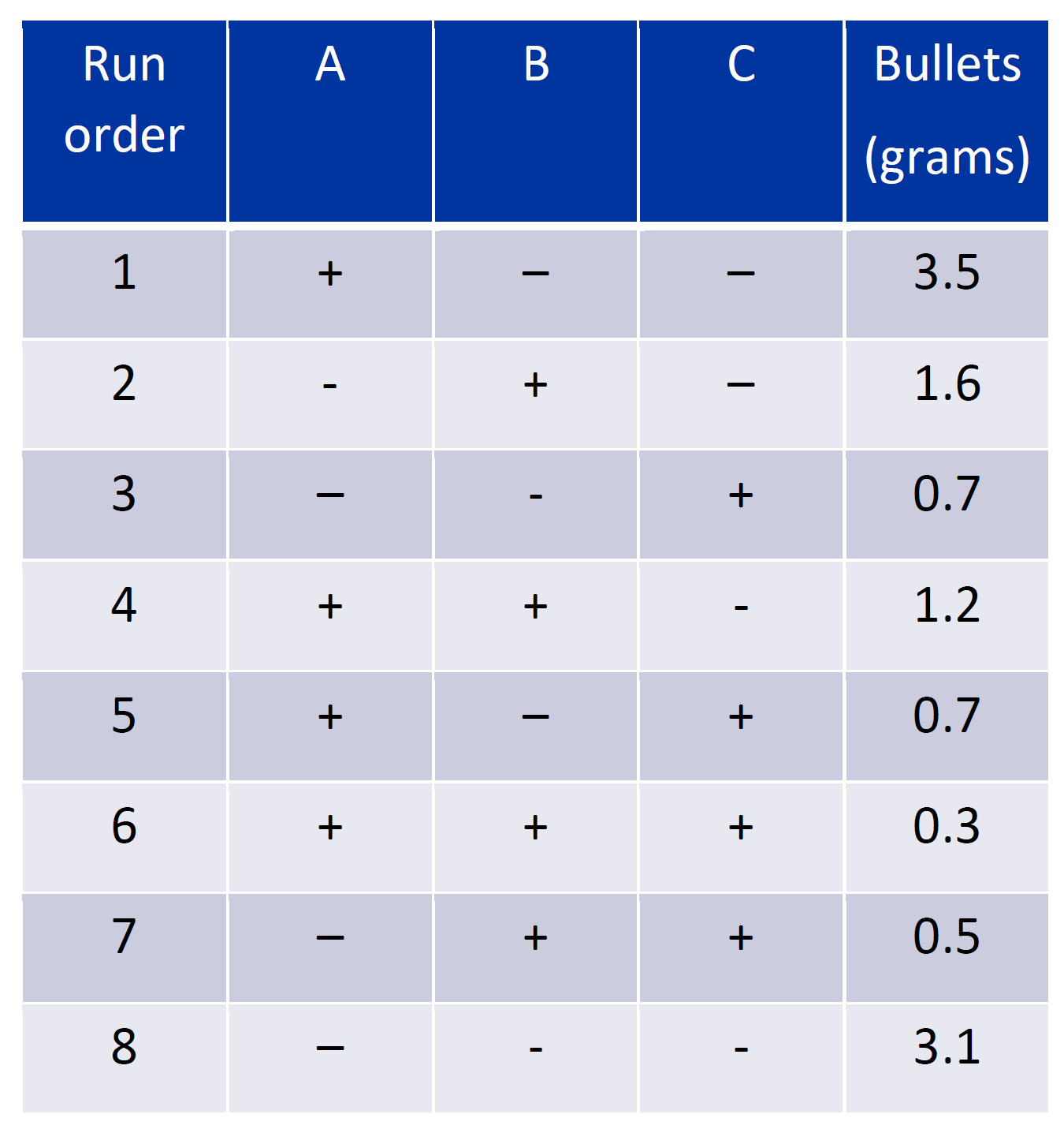
In this blog, I will be documenting the design of experiments, so our task was to document and describe how I did the full and fractional data analysis on the given case study. I am the CEO of the team, and I did case study 1 along with the CFO. Case study 1 is about what causes the loss of popcorn yield when making microwave popcorn.
These are the factors that were identified:
Diameter of bowls to contain the corn, 10 cm and 15 cm (Factor A)
Microwaving time, 4 minutes and 6 minutes (Factor B)
Power setting of microwave, 75% and 100% (Factor C)
8 runs were performed with 100 grams of corn used in every experiment and the measured variable is the amount of “bullets” formed in grams.
Table of Average Mass of Each Run
Full Factorial Design
Effects of Single Factors

These were the values that were keyed into the excel sheet. The given data in the case study was the average of 8 replicates for each run. Therefore, only one value is keyed into the excel sheet.
Table of Average Mass of each Factor at + and at -


From the graph above, it is shown that factor C has the largest gradient which shows it has the largest difference of 1.8g. This means that it has the largest change when the power setting of the microwave is changed from 75% to 100%. It shows that it is the most significant because it has the biggest influence on the reaction, so the higher the power setting, the lesser the mass of bullets. Hence, the higher the popcorn yield. The next factor is B, it has the second largest difference of 1.1g. As microwaving time increases, the mass of bullets decreases. The least significant factor is A, this is because it has the smallest difference of 0.05g.
Ranking of Effect of Single Factors:
1: Factor C
2: Factor B
3: Factor A
Interaction Effects
AxB:
The table below consolidates the values that will provide useful information for the interaction between factors A and B.


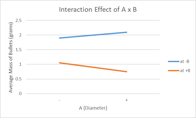
The graph shows that the gradients of both lines are different, one has positive gradient while the other has negative. This shows that there is significant interaction between these two factors due to the difference in the gradients.
AxC:
The table below consolidates the values that will provide useful information for the interaction between factors A and C.


The graph shows a slight difference in the gradients of both lines. This shows that there is interaction between the two factors, however, the interaction is very small.
BxC:


The graph shows that both lines have negative gradients. The difference in the gradients can be considered quite large, therefore it can be considered as significant interaction between these two factors.
In conclusion, for the data analysis for full factorial design, factor C is the most significant factor followed by factor B and A. For the interaction effects between factors, AxB and BxC have the most significant interactions. Therefore, to achieve the best yield of popcorn, factor C has to be at 100% and the most significant interactions between factors can be considered to produce the best popcorn yield.
This is the link to the excel file for the full factorial design:
Fractional Factorial Design
Effect of Single Factors
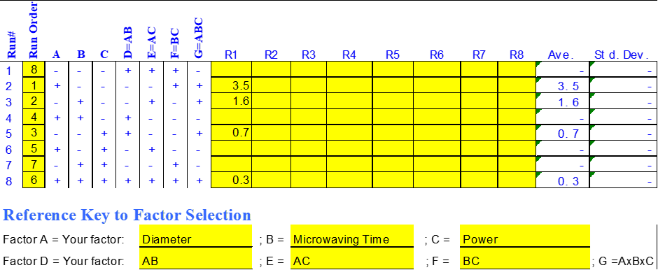
The runs that were chosen for the fractional factorial design are 1, 2, 3, 6 from the run order. This is because these runs provide all factors that occur the same number of times both at high and low levels, thus these runs are orthogonal and will provide good statistical properties.
Table of Average Mass of each Factor at + and at -


From the graph above, it can be determined that factor C is the most significant factor because it has the largest gradient with 1.03g. Therefore, it has the largest changes between high and low. When the power setting of the microwave is increased from 75% to 100%, there will be less bullets in the bowl of popcorn. The next most significant factor is factor B, this is because it has the second largest gradient with 0.58g. Lastly, factor A is the least significant due to its smallest gradient with 0.38g.
Ranking of Effect of Single Factors:
1: Factor C
2: Factor B
3: Factor A
In conclusion, when the runs for the fractional factorial design are chosen correctly, it should also show the same results as in the full factorial design just like this case study. The run order chosen were 1, 2, 3 and 6, they are orthogonal and provide good statistical properties. Therefore, fractional factorial is more efficient because it uses less runs, but the runs have to be chosen correctly.
Comments
Post a Comment